Application: Optimal Growth#
![]()
Exercises from the Class Notes#
Exercise 3.1#
Assume that (A1)-(A3) hold. Which of the assumptions presented in Lectures 1 and 2 are satisfied?
Solution
Assumptions A1.1, A1.2, A2.1, A2.3, and A2.4. In assumption A2.2, \(F\) is not bounded under (A1)-(A3). However, we can assume that capital is at most equal to the maximum maintainable capital stock.
Exercise 3.2#
Show that, for any \(k_0 \in (0,k_{max}]\), the optimal sequence \(\{k_t\}_{t=0}^{\infty}\) defined by \(k_{t+1}=g(k_t)\) converges to \(k^*=f'^{-1}(1/\beta)\).
Solution
From fact that \(v\) is strictly concave, we have
with equality iff \(g\left(k\right) = k\). By the FOC and EC conditions and use the fact that \(U^{'}\left(c\right)>0\), we can conclude that
with equality iff \(g\left(k\right) = k\). Since \(f\) is concave, it follows that \(f^{'}\left(k\right) \stackrel{>}{<} \frac{1}{\beta}\) as \(k\stackrel{<}{>} k^{*}\) and \(k \stackrel{>}{<} g\left(k\right)\) that as \(k \stackrel{>}{<} k^{*}\).
Consider the optimal sequence \(\{k_t\}_{t=0}^{\infty}\) defined by \(k_{t+1}=g(k_t)\). If \(k_{t} \geq k^{*}\), then \(k_{t+1} =g(k_t)\leq k_{t}\) decreases until \(k = k^{*}\). Likewise, if \(k_{t} \leq k^{*}\), then \(k_{t+1}=g(k_t) \geq k_{t}\) increases until \(k = k^{*}\). Therefore the optimal sequence \(\{k_t\}_{t=0}^{\infty}\) converges to \(k^{*}\).
Exercise 3.3#
Write a code in Python that uses an iterative procedure to solve for the value function of the optimal growth model.
Solution
# -*- coding: utf-8 -*-
"""
Created on Sun Nov 18 14:37:30 2018
@author: Bruno
"""

#==============================================================================
# Recursive Methods - Optimal Growth
#==============================================================================

import os
import numpy as np
from scipy.optimize import fminbound


def bellman_operator(w, grid, β, u, f, Tw=None, compute_policy=0):
    # === Apply linear interpolation to w === #
    w_func = lambda x: np.interp(x, grid, w)

    # == Initialize Tw if necessary == #
    if Tw is None:
        Tw = np.empty_like(w)

    if compute_policy:
        σ = np.empty_like(w)

    # == set Tw[i] = max_c { u(c) + β E w(f(y  - c) z)} == #
    for i, y in enumerate(grid):
        def objective(c, y=y):
            # return #Your code goes here
            return - u(c) - β * w_func(f(y - c))
        c_star = fminbound(objective, 1e-10, y)
        if compute_policy:
            # σ[i] = #Your code goes here #y_(t+1) as a function of y_t
            σ[i] = f(y-c_star) #y_(t+1) as a function of y_t
        # Tw[i] = #Your code goes here
        Tw[i] = - objective(c_star)

    if compute_policy:
        return Tw, σ
    else:
        return Tw


def solve_optgrowth(initial_w, grid, β, u, f, tol=1e-4, max_iter=500):

    w = initial_w  # Set initial condition
    error = tol + 1
    i = 0

    # == Create storage array for bellman_operator. Reduces  memory
    # allocation and speeds code up == #
    Tw = np.empty(len(grid))

    # Iterate to find solution
    while error > tol and i < max_iter:
        w_new = bellman_operator(w,
                                 grid,
                                 β,
                                 u,
                                 f,
                                 Tw)
        # error = #Your code goes here
        error = np.max(np.abs(w_new - w))
        w[:] = w_new
        i += 1
        print("Iteration "+str(i)+'\n Error is '+str(error)+'\n') if i % 50 == 0 or error < tol else None


    # Computes policy
    policy = bellman_operator(w,
                             grid,
                             β,
                             u,
                             f,
                             Tw,
                             compute_policy=1)[1]

    return [w, policy]


class CES_OG:
    """
    Constant elasticity of substitution optimal growth model so that

        y = f(k) = k^α


    The class holds parameters and true value and policy functions.
    """

    def __init__(self, α=0.4, β=0.96, sigma=0.9):

        self.α, self.β, self.sigma = α, β, sigma

    def u(self, c):
        " Utility "
        return (c**(1-self.sigma)-1)/(1-self.sigma)

    def f(self, k):
        " Deterministic part of production function.  "
        return k**self.α
# Creation of the model
ces = CES_OG()
# == Unpack parameters / functions for convenience == #
α, β, sigma = ces.α, ces.β, ces.sigma


### Setup of the grid
grid_max = 1         # Largest grid point
grid_size = 200      # Number of grid points
grid = np.linspace(1e-5, grid_max, grid_size)

# Initial conditions and shocks
initial_w = 5 * np.log(grid)


# Computation of the value function
solve = solve_optgrowth(initial_w, grid, β, u=ces.u,
                               f=ces.f, tol=1e-4, max_iter=500)

value_approx = solve[0]
policy_function = solve[1]
Iteration 50
 Error is 0.13013875164658728
Iteration 100
 Error is 0.016903175250330804
Iteration 150
 Error is 0.002195482297175033
Iteration 200
 Error is 0.0002851634526557234
Iteration 226
 Error is 9.866159687632603e-05
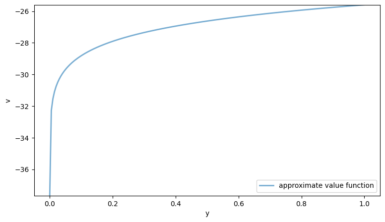
#==============================================================================
# Plotting value function
#==============================================================================
import matplotlib.pyplot as plt

fig, ax = plt.subplots(figsize=(9, 5))
ax.set_ylim(min(value_approx), max(value_approx))
ax.plot(grid, value_approx, lw=2, alpha=0.6, label='approximate value function')
ax.set_xlabel('y')
ax.set_ylabel('v')
ax.legend(loc='lower right')
plt.show()
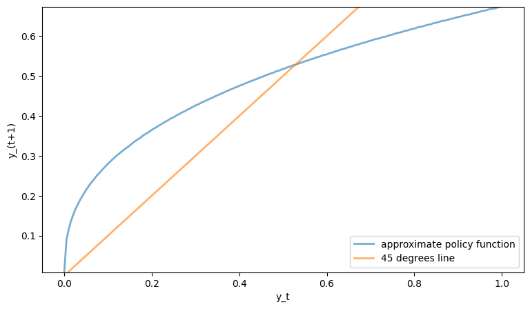
#==============================================================================
# Plotting Policy function
#==============================================================================

fig, ax = plt.subplots(figsize=(9, 5))
ax.set_ylim(min(policy_function), max(policy_function))
ax.plot(grid, policy_function, lw=2, alpha=0.6, label='approximate policy function')

# 45° line
ax.plot(grid, grid, lw=2, alpha=0.6, label='45 degrees line')

ax.set_xlabel('y_t')
ax.set_ylabel('y_(t+1)')
ax.legend(loc='lower right')
plt.show()
Additional Exercises#
Exercise 3.4 (Sufficiency of Euler and transversality conditions)#
Assume that the Assumptions in Lecture 2 are satisfied.
Show that the sequence \(\{x^*_{t+1}\}_{t=0}^{\infty}\) with \(x^*_{t+1}\in\Gamma(x_t)\) for all \(t\geq 0\), is optimal for the Sequential Problem if it satisfies the Euler equation and the following transversality condition: \(\lim_{t\rightarrow \infty} \beta^t F_1(x^*_{t},x^*_{t+1})\cdot x^*_{t}=0\).
Can we replace the transversality condition in 1 with that of the recursive problem: \(\lim_{t\rightarrow \infty} \beta^t V(x^*_{t})=0\)?
Solution
It is sufficient to show that the difference between the objective function in the sequential problem evaluated at \(\{x^{*}\}\) and at \(\{x_{t}\}\) is nonnegative.
Since \(F\) is continuous, concave, and differentiable,
Since \(x_{0}^{*} - x_{0} = 0\), rearranging terms givees
Since \(\{x^{*}\}\) satisfies the FOC, the terms in the summation are all zero. Therefore, by the FOC and using the Euler Equation to substitute the last remaining term, we obtain
It then follows that \(D\geq 0\), establishing the desired result.
Yes, because the value function is concave in this setting.
Exercise 3.5#
Let \(\bar{k}=f(\bar{k})\) denote the maximum maintainable capital stock. Show that the standard assumptions on \(f\) and \(U\) ensure that for any \(k\in(0,\bar{k}]\), the solution of the Bellman equation is at an interior value for \(k'\), so that \(v\) is continuously differentiable on \((0,\bar{k}]\), and that the FOC and Envelope Condition (EC) hold for all \(k\in(0,\bar{k}]\).
Use the EC to show that the policy function \(g(k)\) is strictly increasing.
Solution
Pick any \(k\in (0,\overline{k}]\). To see that \(g\left(k\right) \in \left(0,\overline{k}\right)\), suppose \(g\left(k\right) = 0\). Then,
but the left-hand side is finite while the right-had side is not. There \(k\left(k\right) = 0\) cannot not be optimal.
Suppose then \(g\left(k\right) = \overline{k}\). Because \(k\in (0,\overline{k}]\), and consumption is nonnegative, it must be that \(k = \overline{k}\). Hence,
but the left-hand side of the inequality stated above is not finite. On the other hand, feasibility requires that \(g\left(\overline{k}\right)\leq \overline{k}\). If \(g\left(\overline{k}\right)= \overline{k}\), this implies zero consumption even after, which is suboptimal. Hence \(g\left(\overline{k}\right)< \overline{k}\). But
and the right-hand side is finite, which is a contradiction. Therefore, the solution of the Bellman equation is an interior value for \(k^{'}\). By Theorem 4.11 (Differentiability of the value function), v is contiunously differentiable on \((0,\overline{k}]\).
Pick \(k,\ k^{'}\in (0,\overline{k}]\), with \(k<k^{'}\). Suppose \(g\left(k\right)\geq g\left(k^{'}\right)\). Then \(v\) being strictly concave implies
Hence, by \(U\) being strictly concave,
Then, \(f\) being strictily increasing implies
and so \(g\left(k^{'}\right)>g\left(k\right)\), which is a contraction.
Exercise 3.6#
Consider a modification of the canonical growth model where capital goods are produced using only labor. We endow the consumer with one unit labor, and assume that \(c_t=n_tf(k_t/n_t) \text{ and } k_{t+1}=1-n_t.\) We also assume that \(\lim_{n\rightarrow 0} nf(k,n)=0\) for all \(k\in[0,1]\).
Write the Bellman equation. Derive the FOC and EC.
Find a necessary condition that must be satisfied by the stationary capital stock. Prove that it indeed identifies the steady-state.
Let \(U(c)=c^{\alpha}\) with \(\alpha \in (0,1)\) and \(f(x)=x^{\theta}\) with \(\theta \in (0,1)\). Use the FOC to show that the policy function \(g(k)\) is strictly decreasing on \([0,1]\).
Solution
The Bellman equation can be written as
Let \(g\) denote the policy funtion. The first-order and envelope conditions are given by
Setting \(g\left(k_{t}\right) = k_{t}\) and eliminating \(k_{t}^{'}\), a necessary condition for a stationary point is
By the assumptions on \(f\), the equation above has exactly one solution, denoted as \(k^{*}\). Since \(v\) is strictly concave, the condition in Exercise 3.2 holds. Substituting from the FOC and EC, we have
with equality only if \(g\left(k_{t}\right) = k_{t}\). Therefore \(k^{*}\) is indeed a stationary point.
Pick \(k,\ k^{'}\in (0,\overline{k}]\), with \(k<k^{'}\). Suppose \(g\left(k\right)\geq g\left(k^{'}\right)\). With the specific function forms, the FOC is given by
As \(v\) is strictly concave, we have
which implies
where
Hence,
and so \(g\left(k^{'}\right)<g\left(k\right)\), which is a contradiction.
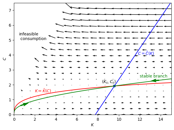
Phase Diagram#
The code below is borrowed from QuantEcon
It displays the phase diagram of the infinite horizon growth model when
Utility function is CRRA: \(U(c)=\frac{c^{1-\gamma}}{1-\gamma}\);
Production function is Cobb-Douglas with fixed labor supply: \(F(K,1)=K^{\alpha}\).
import matplotlib.pyplot as plt
from numba import njit, float64
from numba.experimental import jitclass
import numpy as np
from quantecon.optimize import brentq
We first define a jitclass that stores parameters and functions that define our economy.
planning_data = [
    ('γ', float64),    # Coefficient of relative risk aversion
    ('β', float64),    # Discount factor
    ('δ', float64),    # Depreciation rate on capital
    ('α', float64),    # Return to capital per capita
    ('A', float64)     # Technology
]
@jitclass(planning_data)
class PlanningProblem():

    def __init__(self, γ=2, β=0.95, δ=0.02, α=0.33, A=1):

        self.γ, self.β = γ, β
        self.δ, self.α, self.A = δ, α, A

    def u(self, c):
        '''
        Utility function
        ASIDE: If you have a utility function that is hard to solve by hand
        you can use automatic or symbolic differentiation
        See https://github.com/HIPS/autograd
        '''
        γ = self.γ

        return c ** (1 - γ) / (1 - γ) if γ!= 1 else np.log(c)

    def u_prime(self, c):
        'Derivative of utility'
        γ = self.γ

        return c ** (-γ)

    def u_prime_inv(self, c):
        'Inverse of derivative of utility'
        γ = self.γ

        return c ** (-1 / γ)

    def f(self, k):
        'Production function'
        α, A = self.α, self.A

        return A * k ** α

    def f_prime(self, k):
        'Derivative of production function'
        α, A = self.α, self.A

        return α * A * k ** (α - 1)

    def f_prime_inv(self, k):
        'Inverse of derivative of production function'
        α, A = self.α, self.A

        return (k / (A * α)) ** (1 / (α - 1))

    def next_k_c(self, k, c):
        ''''
        Given the current capital Kt and an arbitrary feasible
        consumption choice Ct, computes Kt+1 by state transition law
        and optimal Ct+1 by Euler equation.
        '''
        β, δ = self.β, self.δ
        u_prime, u_prime_inv = self.u_prime, self.u_prime_inv
        f, f_prime = self.f, self.f_prime

        k_next = f(k) + (1 - δ) * k - c
        c_next = u_prime_inv(u_prime(c) / (β * (f_prime(k_next) + (1 - δ))))

        return k_next, c_next
# Create economy instance
pp = PlanningProblem()
# Compute stable manifold for Consumption
@njit
def C_tilde(K, pp):

    return pp.f(K) + (1 - pp.δ) * K - pp.f_prime_inv(1 / pp.β - 1 + pp.δ)

# Compute stable manifold for Capital
@njit
def K_diff(K, C, pp):

    return pp.f(K) - pp.δ * K - C

@njit
def K_tilde(C, pp):

    res = brentq(K_diff, 1e-6, 100, args=(C, pp))

    return res.root
# Compute steady-state by combining the two stable manifolds
@njit
def K_tilde_diff(K, pp):

    K_out = K_tilde(C_tilde(K, pp), pp)

    return K - K_out

res = brentq(K_tilde_diff, 8, 10, args=(pp,))

Ks = res.root
Cs = C_tilde(Ks, pp)

Ks, Cs
# Implements the shooting algorithm for the planning problem.
@njit
def shooting(pp, c0, k0, T=10):
    '''
    Given the initial condition of capital k0 and an initial guess
    of consumption c0, computes the whole paths of c and k
    using the state transition law and Euler equation for T periods.
    '''
    if c0 > pp.f(k0) + (1 - pp.δ) * k0:
        print("initial consumption is not feasible")

        return None

    # initialize vectors of c and k
    c_vec = np.empty(T+1)
    k_vec = np.empty(T+2)

    c_vec[0] = c0
    k_vec[0] = k0

    for t in range(T):
        k_vec[t+1], c_vec[t+1] = pp.next_k_c(k_vec[t], c_vec[t])

    k_vec[T+1] = pp.f(k_vec[T]) + (1 - pp.δ) * k_vec[T] - c_vec[T]

    return c_vec, k_vec
# Use a bisection method to match the terminal condition
@njit
def bisection(pp, c0, k0, T=10, tol=1e-4, max_iter=500, k_ter=0, verbose=True):

    # initial boundaries for guess c0
    c0_upper = pp.f(k0)
    c0_lower = 0

    i = 0
    while True:
        c_vec, k_vec = shooting(pp, c0, k0, T)
        error = k_vec[-1] - k_ter

        # check if the terminal condition is satisfied
        if np.abs(error) < tol:
            if verbose:
                print('Converged successfully on iteration ', i+1)
            return c_vec, k_vec

        i += 1
        if i == max_iter:
            if verbose:
                print('Convergence failed.')
            return c_vec, k_vec

        # if iteration continues, updates boundaries and guess of c0
        if error > 0:
            c0_lower = c0
        else:
            c0_upper = c0

        c0 = (c0_lower + c0_upper) / 2
We now compute two trajectories towards the steady-state that start from different sides of K_{S}.
c_vec1, k_vec1 = bisection(pp, 5, 15, T=200, k_ter=Ks)
c_vec2, k_vec2 = bisection(pp, 1e-3, 1e-3, T=200, k_ter=Ks)
# Plot Phase Diagram
fig, ax = plt.subplots(figsize=(7, 5))

K_range = np.arange(1e-1, 15, 0.1)
C_range = np.arange(1e-1, 2.3, 0.1)

# C tilde
ax.plot(K_range, [C_tilde(Ks, pp) for Ks in K_range], color='b')
ax.text(11.8, 4, r'$C=\tilde{C}(K)$', color='b')

# K tilde
ax.plot([K_tilde(Cs, pp) for Cs in C_range], C_range, color='r')
ax.text(2, 1.5, r'$K=\tilde{K}(C)$', color='r')

# stable branch
ax.plot(k_vec1[:-1], c_vec1, color='g')
ax.plot(k_vec2[:-1], c_vec2, color='g')
ax.quiver(k_vec1[5], c_vec1[5],
          k_vec1[6]-k_vec1[5], c_vec1[6]-c_vec1[5],
          color='g')
ax.quiver(k_vec2[5], c_vec2[5],
          k_vec2[6]-k_vec2[5], c_vec2[6]-c_vec2[5],
          color='g')
ax.text(12, 2.5, r'stable branch', color='g')

# (Ks, Cs)
ax.scatter(Ks, Cs)
ax.text(Ks-1.2, Cs+0.2, '$(K_s, C_s)$')

# arrows
K_range = np.linspace(1e-3, 15, 20)
C_range = np.linspace(1e-3, 7.5, 20)
K_mesh, C_mesh = np.meshgrid(K_range, C_range)

next_K, next_C = pp.next_k_c(K_mesh, C_mesh)
ax.quiver(K_range, C_range, next_K-K_mesh, next_C-C_mesh)

# infeasible consumption area
ax.text(0.5, 5, "infeasible\n consumption")

ax.set_ylim([0, 7.5])
ax.set_xlim([0, 15])

ax.set_xlabel('$K$')
ax.set_ylabel('$C$')

plt.show()